Regression Review

In this application exercise we will be studying loan interest rates. The dataset is one you’ve come across before in your reading – the dataset about loans from the peer-to-peer lender, Lending Club, from the openintro package. We will use tidyverse and tidymodels for data exploration and modeling, respectively.

library(tidyverse)
library(tidymodels)
library(openintro)

Before we use the data set, we’ll make a few transformations to it.

Warm up: What is this code doing?

loans <- loans_full_schema %>% # Old data set
  mutate(
    credit_util = total_credit_utilized / total_credit_limit, #New var
    bankruptcy  = as.factor(if_else(public_record_bankrupt == 0, 0, 1)),
    verified_income = droplevels(verified_income),
    homeownership = str_to_title(homeownership),
    homeownership = fct_relevel(homeownership, "Rent", "Mortgage", "Own")
    ) %>%
  rename(credit_checks = inquiries_last_12m) %>%
  select(interest_rate, verified_income, debt_to_income, credit_util, bankruptcy, term, credit_checks, issue_month, homeownership)

Take a glimpse of the data below:

glimpse(loans)

Rows: 10,000
Columns: 9
$ interest_rate   <dbl> 14.07, 12.61, 17.09, 6.72, 14.07, 6.72, 13.59, 11.99, …
$ verified_income <fct> Verified, Not Verified, Source Verified, Not Verified,…
$ debt_to_income  <dbl> 18.01, 5.04, 21.15, 10.16, 57.96, 6.46, 23.66, 16.19, …
$ credit_util     <dbl> 0.54759517, 0.15003472, 0.66134832, 0.19673228, 0.7549…
$ bankruptcy      <fct> 0, 1, 0, 0, 0, 0, 0, 0, 0, 0, 1, 0, 0, 0, 1, 0, 0, 0, …
$ term            <dbl> 60, 36, 36, 36, 36, 36, 60, 60, 36, 36, 60, 60, 36, 60…
$ credit_checks   <int> 6, 1, 4, 0, 7, 6, 1, 1, 3, 0, 4, 4, 8, 6, 0, 0, 4, 6, …
$ issue_month     <fct> Mar-2018, Feb-2018, Feb-2018, Jan-2018, Mar-2018, Jan-…
$ homeownership   <fct> Mortgage, Rent, Rent, Rent, Rent, Own, Mortgage, Mortg…

Interest rate vs. credit utilization ratio

Write a model that models interest rate by credit utilization ratio. Name it rate_util_fit.

rate_util_fit <- linear_reg() |>
  set_engine("lm") |>
  fit(interest_rate ~ credit_util, data = loans) 
  
tidy(rate_util_fit)

# A tibble: 2 × 5
  term        estimate std.error statistic   p.value
  <chr>          <dbl>     <dbl>     <dbl>     <dbl>
1 (Intercept)    10.5     0.0871     121.  0        
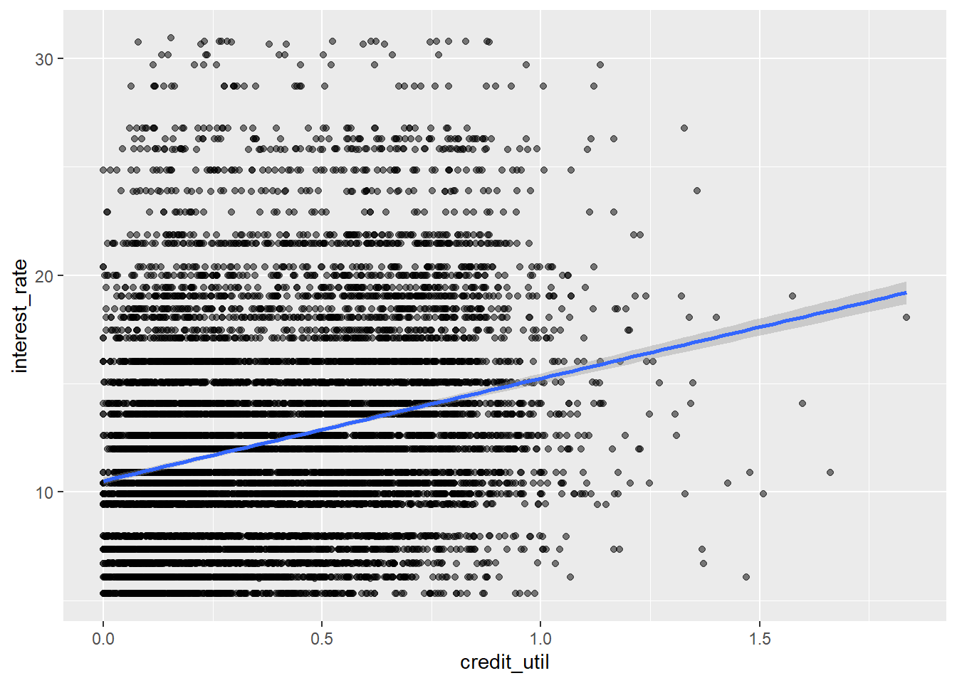
2 credit_util     4.73    0.180       26.3 1.18e-147

And here is the model visualized:

ggplot(loans, aes(x = credit_util, y = interest_rate)) +
  geom_point(alpha = 0.5) +
  geom_smooth(method = "lm")

`geom_smooth()` using formula 'y ~ x'

Warning: Removed 2 rows containing non-finite values (stat_smooth).

Warning: Removed 2 rows containing missing values (geom_point).

Your turn: What is the estimated interest rate for a loan applicant with credit utilization of 0.8, i.e. someone whose total credit balance is 80% of their total available credit?

# Make new data 

credit_util_80 <- tibble(credit_util = 0.8)

# Predict with it

predict(rate_util_fit, new_data = credit_util_80)

# A tibble: 1 × 1
  .pred
  <dbl>
1  14.3

Leverage vs Influence

What is leverage? What is influence?

Leverage - How far away an observation is from the line (High, Low) “Potential for influence”

Influence - Does the observation change the line?

Now, let’s add data points to drive this idea home!

new_point_1 <- data.frame(100, NA, NA, 0.8, NA,  NA, NA, NA, NA)
names(new_point_1) <- names(loans)

new_point_2 <- data.frame(100, NA, NA, 4, NA,  NA, NA, NA, NA)
names(new_point_2) <- names(loans)


new_loans1 <- rbind(loans, new_point_1)

new_loans2 <- rbind(loans, new_point_2)

Below, compare the model outputs.

linear_reg() |>
  set_engine("lm") |>
  fit(interest_rate ~ credit_util, data = loans) |> #Change data to loans
  tidy()

# A tibble: 2 × 5
  term        estimate std.error statistic   p.value
  <chr>          <dbl>     <dbl>     <dbl>     <dbl>
1 (Intercept)    10.5     0.0871     121.  0        
2 credit_util     4.73    0.180       26.3 1.18e-147

linear_reg() |>
  set_engine("lm") |>
  fit(interest_rate ~ credit_util, data = new_loans1) |>
  tidy()

# A tibble: 2 × 5
  term        estimate std.error statistic   p.value
  <chr>          <dbl>     <dbl>     <dbl>     <dbl>
1 (Intercept)    10.5     0.0884     119.  0        
2 credit_util     4.77    0.182       26.2 3.94e-146

linear_reg() |>
  set_engine("lm") |>
  fit(interest_rate ~ credit_util, data = new_loans2) |>
  tidy()

# A tibble: 2 × 5
  term        estimate std.error statistic   p.value
  <chr>          <dbl>     <dbl>     <dbl>     <dbl>
1 (Intercept)    10.4     0.0875     119.  0        
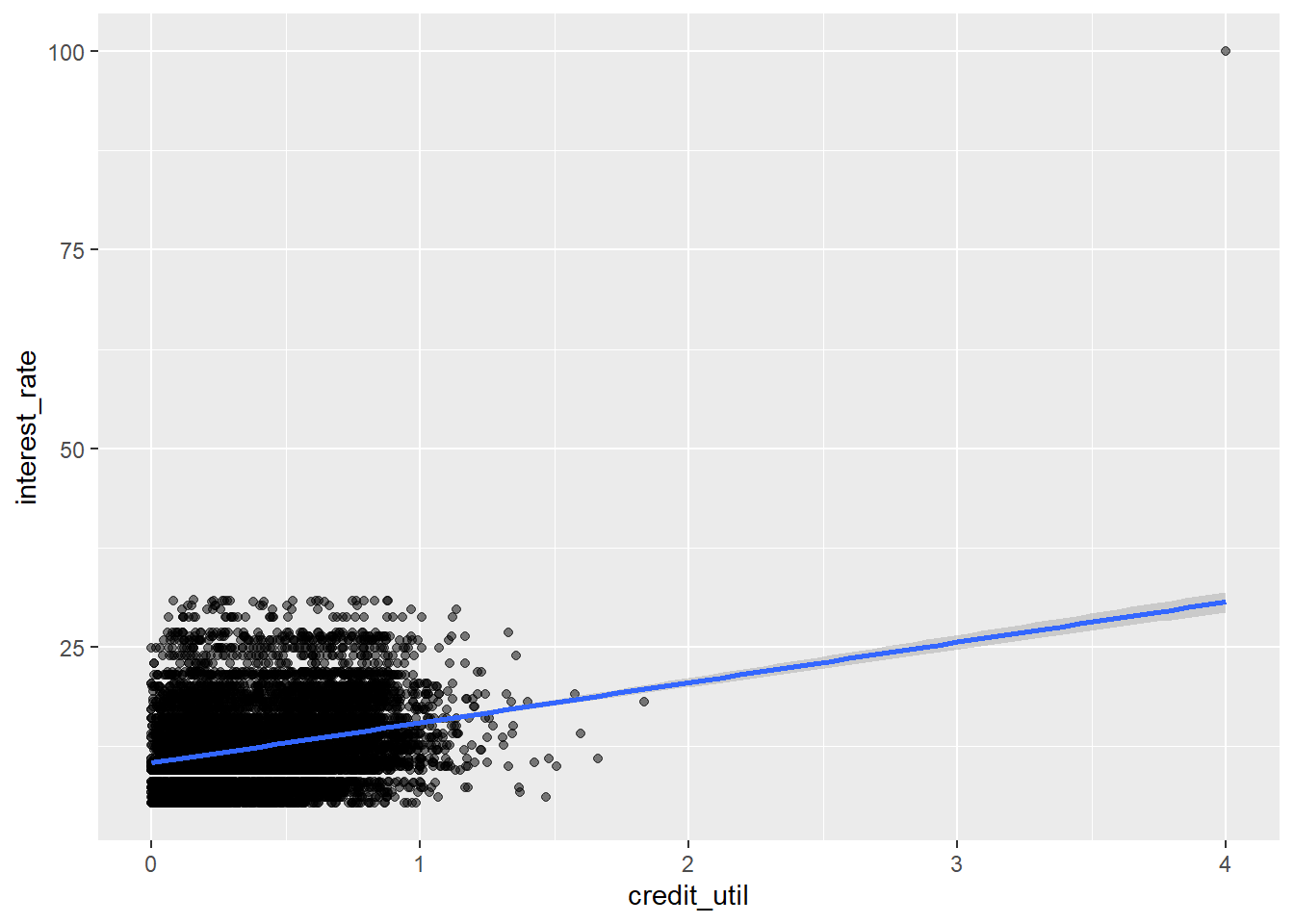
2 credit_util     5.07    0.180       28.2 2.54e-168

ggplot(new_loans2, aes(x = credit_util, y = interest_rate)) +
  geom_point(alpha = 0.5) +
  geom_smooth(method = "lm")

`geom_smooth()` using formula 'y ~ x'

Warning: Removed 2 rows containing non-finite values (stat_smooth).

Warning: Removed 2 rows containing missing values (geom_point).

Model 3 had its slope change dramatically because of the high leverage point with a large x-value and large y-value. The slope did not change in model 2 very much compared to model 1

Interest rate vs. homeownership

Next lets predict interest rates from homeownership, which is a categorical predictor with three levels:

levels(loans$homeownership)

[1] "Rent"     "Mortgage" "Own"

Demo: Fit the linear regression model to predict interest rate from homeownership and display a tidy summary of the model. Write the estimated model output below.

rate_util_home_fit <- linear_reg() |>
  set_engine("lm") |>
  fit(interest_rate ~ homeownership, data = loans)

tidy(rate_util_home_fit)

# A tibble: 3 × 5
  term                  estimate std.error statistic  p.value
  <chr>                    <dbl>     <dbl>     <dbl>    <dbl>
1 (Intercept)             12.9      0.0803    161.   0       
2 homeownershipMortgage   -0.866    0.108      -8.03 1.08e-15
3 homeownershipOwn        -0.611    0.158      -3.88 1.06e- 4

Your turn: Interpret each coefficient in context of the problem.
- Intercept: On average, the estimated interest rate for a house being rented is 12.9 percent.
- Slopes:
  - On average, the estimated interest rate for a mortgage is 12.9 - 0.866 percent.
  - On average, the estimated interest rate for a owned home is 12.9 - 0.611 percent.

Interest rate vs. credit utilization and homeownership

Main effects model

Demo: Fit a model to predict interest rate from credit utilization and homeownership, without an interaction effect between the two predictors. Display the summary output and write out the estimated regression equation.

rate_util_home_fit <- linear_reg() |>
  fit(interest_rate ~ credit_util + homeownership, data = loans)
tidy(rate_util_home_fit)

# A tibble: 4 × 5
  term                  estimate std.error statistic   p.value
  <chr>                    <dbl>     <dbl>     <dbl>     <dbl>
1 (Intercept)              9.93      0.140    70.8   0        
2 credit_util              5.34      0.207    25.7   2.20e-141
3 homeownershipMortgage    0.696     0.121     5.76  8.71e-  9
4 homeownershipOwn         0.128     0.155     0.827 4.08e-  1

= 9.93 + 5.34 credit-util + 0.696Mortgage + 0.128Own \

Mortage = 1 if Mortage; 0 else \ Own = 1 if Own; 0 else

Demo: Write the estimated regression equation for loan applications from each of the homeownership groups separately.
- Rent: $ = 9.93 + 5.34 credit-util \ $
- Mortgage: $ = 9.93 + 5.34 credit-util + 0.696*(1) \ $
- Own: $ = 9.93 + 5.34 credit-util + 0.128*(1) \ $
Question: How does the model predict the interest rate to vary as credit utilization varies for loan applicants with different homeownership status. Are the rates the same or different?

The Same

Interaction effects model

Demo: Fit a model to predict interest rate from credit utilization and homeownership, with an interaction effect between the two predictors. Display the summary output and write out the estimated regression equation.

rate_util_home_int_fit <- linear_reg() |>
  set_engine("lm") |> 
  fit(interest_rate ~ homeownership*credit_util, data = loans)
  
  tidy(rate_util_home_int_fit)

# A tibble: 6 × 5
  term                              estimate std.error statistic  p.value
  <chr>                                <dbl>     <dbl>     <dbl>    <dbl>
1 (Intercept)                          9.44      0.199     47.5  0       
2 homeownershipMortgage                1.39      0.228      6.11 1.04e- 9
3 homeownershipOwn                     0.697     0.316      2.20 2.75e- 2
4 credit_util                          6.20      0.325     19.1  1.01e-79
5 homeownershipMortgage:credit_util   -1.64      0.457     -3.58 3.49e- 4
6 homeownershipOwn:credit_util        -1.06      0.590     -1.80 7.24e- 2

\[ \widehat{interest~rat e} = 9.44 + 6.20 \times credit\_util + 1.39 \times Mortgage + 0.697 \times Own - 1.64 \times credit\_util:Mortgage - 1.06 \times credit\_util:Own \]

Demo: Write the estimated regression equation for loan applications from each of the homeownership groups separately.
- Rent: $\widehat{interest~rate} = 9.44 + 6.20 \times credit~util$
- Mortgage: $\widehat{interest~rate} = 10.83 + 4.56 \times credit~util$
- Own: $\widehat{interest~rate} = 10.137 + 5.14 \times credit~util$
Question: How does the model predict the interest rate to vary as credit utilization varies for loan applicants with different homeownership status. Are the rates the same or different?

They are different

Choosing a model

Rule of thumb: Occam’s Razor - Don’t overcomplicate the situation! We prefer the simplest best model.

glance(rate_util_home_fit)

# A tibble: 1 × 12
  r.squared adj.r.…¹ sigma stati…²   p.value    df  logLik    AIC    BIC devia…³
      <dbl>    <dbl> <dbl>   <dbl>     <dbl> <dbl>   <dbl>  <dbl>  <dbl>   <dbl>
1    0.0682   0.0679  4.83    244. 1.25e-152     3 -29926. 59861. 59897. 232954.
# … with 2 more variables: df.residual <int>, nobs <int>, and abbreviated
#   variable names ¹adj.r.squared, ²statistic, ³deviance

glance(rate_util_home_int_fit)

# A tibble: 1 × 12
  r.squared adj.r.…¹ sigma stati…²   p.value    df  logLik    AIC    BIC devia…³
      <dbl>    <dbl> <dbl>   <dbl>     <dbl> <dbl>   <dbl>  <dbl>  <dbl>   <dbl>
1    0.0694   0.0689  4.83    149. 4.79e-153     5 -29919. 59852. 59903. 232652.
# … with 2 more variables: df.residual <int>, nobs <int>, and abbreviated
#   variable names ¹adj.r.squared, ²statistic, ³deviance

Review: What is R-squared? What is adjusted R-squared?

R-squared is the amount of variability in our response that is explained by our model

Adjusted R-squared is similar, but has an additional penalty for the number of variables in the model.

Question: Based on the $R^2s$ of these two models, which one do we prefer? Is this appropriate?
Question: Based on the adjusted $R^2$s of these two models, which one do we prefer?

Note: We can use the principles of adjusted R-squared to select models using forwards or backwards selection (Read 8.4.1)

Another model to consider

Your turn: Let’s add one more model to the variable – issue month. Should we add this variable to the interaction effects model from earlier?

linear_reg() |>
  fit(interest_rate ~ credit_util * homeownership + issue_month, data = loans) |>
  glance()

# A tibble: 1 × 12
  r.squared adj.r.…¹ sigma stati…²   p.value    df  logLik    AIC    BIC devia…³
      <dbl>    <dbl> <dbl>   <dbl>     <dbl> <dbl>   <dbl>  <dbl>  <dbl>   <dbl>
1    0.0694   0.0688  4.83    106. 5.62e-151     7 -29919. 59856. 59921. 232641.
# … with 2 more variables: df.residual <int>, nobs <int>, and abbreviated
#   variable names ¹adj.r.squared, ²statistic, ³deviance

No, the adjusted R-squared went slightly down

Optional

2 Quantitative Explanatory Variables

Remember the penguins? Let’s finish the activity.

Now, let’s explore body mass, and it’s relationship to bill length and flipper length.

library(palmerpenguins)
library(plotly)
library(widgetframe)

Note: This code is beyond the scope of this course!

quanplot <- plot_ly(penguins, 
                    x = ~ flipper_length_mm, y = ~ bill_length_mm, z = ~body_mass_g,
                    marker = list(size = 3, color = "lightgray" , alpha = 0.5, 
                                  line = list(color = "gray" , width = 2))) |>
                      add_markers() |>
                      plotly::layout(scene = list(
                        xaxis = list(title = "Flipper (mm)"),
                        yaxis = list(title = "Bill (mm)"), 
                        zaxis = list(title = "Body Mass (g)")
                      )) |>
                    config(displayModeBar = FALSE)
                  frameWidget(quanplot)

Warning: Ignoring 2 observations

– Fit the additive model below. Interpret the coefficient for flipper in context of the problem.

linear_reg() |>
  set_engine("lm") |>
  fit(body_mass_g ~ bill_length_mm * flipper_length_mm , data = penguins) |>
  tidy()

# A tibble: 4 × 5
  term                             estimate std.error statistic  p.value
  <chr>                               <dbl>     <dbl>     <dbl>    <dbl>
1 (Intercept)                       5091.    2925.        1.74  0.0827  
2 bill_length_mm                    -229.      63.4      -3.61  0.000347
3 flipper_length_mm                   -7.31    15.0      -0.486 0.627   
4 bill_length_mm:flipper_length_mm     1.20     0.322     3.72  0.000232

= -5737 + 6.05bill + 48.1flipper

Holding bill length constant, for a one mm increase in flipper length, we expect on average a 48.1 increase in body mass grams.

What if I want to fit an interaction model with these two quantitative variables?

It looks really similar to what we’ve done before! Try it out!